(Congestion + Volume, 15-60 Minutes Ahead)


PREFACE
Over the last little while I learned two things:
- Edmonton has more traffic sensors than I expected.
- Graph neural networks will humble you repeatedly, and they do it with the calm indifference of an error message.
This project started as “I want to forecast congestion.” It turned into SSL certificates, missing files, broken deployments, baselines that refused to be beaten, and a map full of dots that only looked meaningful after I stared long enough.
ABSTRACT
Traffic is a graph problem that is often treated like a collection of independent time series. In reality, flow and congestion propagate through space: upstream changes appear downstream, and nearby corridors share load during transitions.
In this work, I build a spatio-temporal graph neural network (GNN) pipeline to forecast Edmonton traffic volume and a congestion proxy 15-60 minutes ahead using City of Edmonton sensor data aggregated into 15-minute intervals. Sensors are modeled as nodes; edges are defined by geographic proximity using k-nearest neighbors; temporal evolution is modeled with a recurrent unit over historical windows.
The main result is blunt: the system produces forecasts, but it does not meaningfully outperform a persistence baseline at short horizons. Residual forecasting (predicting deviations from the last observed value) yields small improvements at longer horizons and during rush hour, but the overall gains are marginal. The project mostly demonstrates how hard it is to extract signal beyond “the next hour resembles the last 15 minutes,” especially with limited data and an approximate graph.
INTRODUCTION
Forecasting traffic sounds simple: predict what happens in the next hour. In practice, traffic exhibits strong periodicity (commute cycles), abrupt exogenous shocks (incidents, weather), and spatial coupling (bottlenecks spill, routes substitute).
Many baseline approaches treat each sensor independently. That is workable, but it ignores the spatial structure implied by the road system. A slowdown is rarely isolated.
GNNs provide a way to learn from relational structure while modeling temporal dynamics. The goal here was straightforward:
- Ingest Edmonton traffic sensor data
- Build a graph of sensor sites
- Forecast volume and congestion 15-60 minutes ahead
- Visualize forecasts on a map and rank likely “worst soon” sites
It mostly worked, in the sense that the pipeline runs. It mostly failed, in the sense that the city does not care.
BACKGROUND
Graphs encode entities (nodes) and relationships (edges). In this project:
- Nodes: traffic monitoring sites
- Edges: nearby sensors (k-nearest neighbors using latitude/longitude)
- Features: traffic measurements per 15-minute interval (volume + congestion proxy + time encodings)
- Targets: multi-step future values
A simple GCN update can be written as:
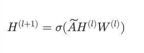
where A_tilde is a normalized adjacency matrix, H is the node representation matrix, W are learnable weights, and sigma is a nonlinearity.
Traffic forecasting also requires time modeling. Spatial edges define possible influence; temporal structure defines when influence matters.
DATA
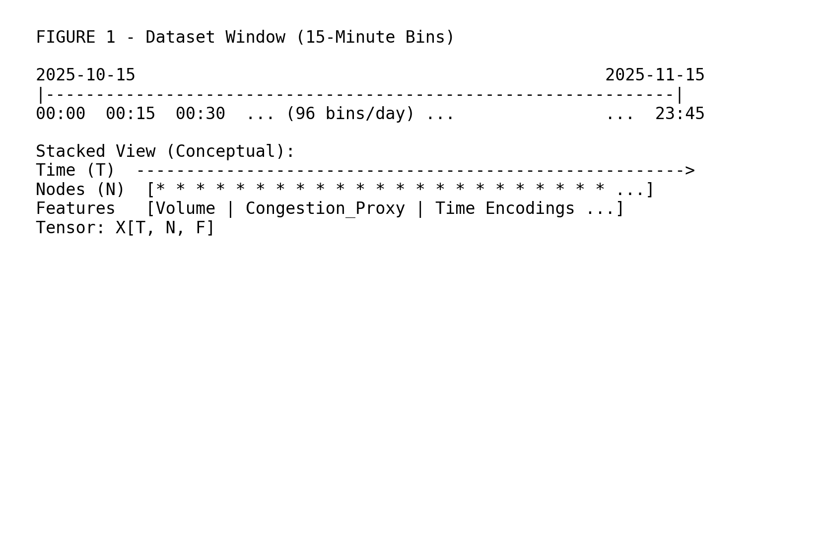
I used City of Edmonton open data traffic sensor records aggregated into 15-minute bins. Each row corresponds to a sensor site and time interval.
I constructed a tensor:
X in R^(T x N x F)
where:
- T is the number of time steps
- N is the number of sensor nodes (approx 225 retained)
- F is the number of features (volume, congestion proxy, time encodings)
I trained on a window like 2025-10-15 -> 2025-11-15. A month of data is enough to learn daily cycles. It is not enough to learn the city’s rare moods.
GRAPH CONSTRUCTION
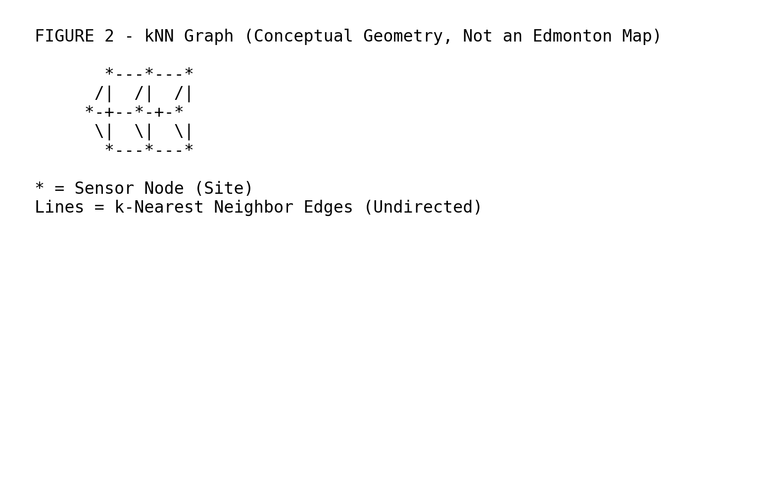
I did not reconstruct the road network. Instead, I used a pragmatic geographic graph:
- Compute pairwise distances from sensor latitude/longitude
- Connect each node to its k nearest neighbors
- k = 8, undirected edges
This graph is a convenience approximation: it encodes local correlation, not actual connectivity.
Conceptually, the graph looks like a local neighborhood mesh: each site is tethered to a small ring of nearby sites, forming overlapping clusters.
Nodes: {v1, v2, …, vN} Edges: (vi, vj) if vj is in kNN(vi)
MODEL
Baseline: Persistence
The persistence model predicts the last observed value:
x_hat(t+h) = x(t)
It is simple and extremely strong for short horizons.
Attempt 1: Direct Forecasting
The first model predicted absolute future values directly using a spatio-temporal architecture (GCN + temporal component). Training behavior looked reasonable: loss decreased and gradients behaved.
Performance did not. MAE was worse than persistence, especially at 15 minutes. The model learned to be confident about being slightly wrong.
Residual Forecasting
To avoid wasting capacity on learning continuity, I switched to residual prediction:
x_hat(t+h) = x(t) + delta(t+h)
where the network outputs delta(t+h).
This reframes the task: persistence is treated as the default, and the model learns corrections during transitions (ramp-up, ramp-down) and spatial spillover.
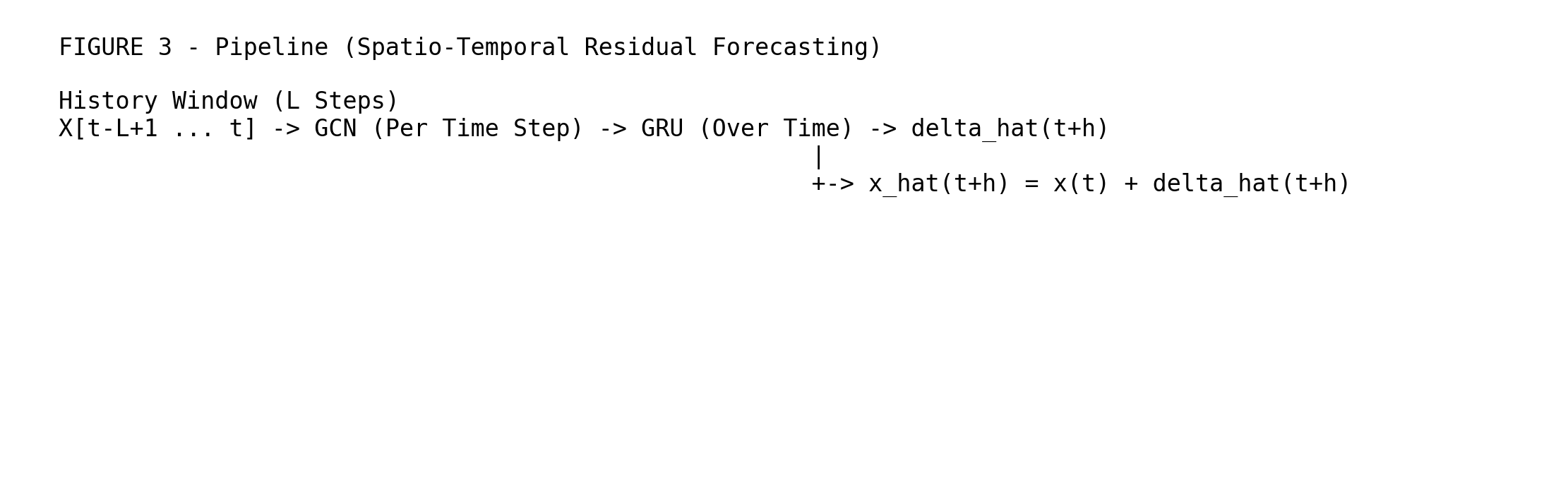
ARCHITECTURE
Spatio-Temporal Residual Model (GCN + GRU)
Given a history window of length L:
- Apply graph convolution at each time step (spatial mixing)
- Feed per-node embeddings through a GRU across time (temporal state)
- Output delta for multiple horizons (15/30/45/60 minutes)
EXPERIMENTS
Setup
- Horizons: 15, 30, 45, 60 minutes
- Metric: MAE (raw units)
- Additional slices: rush-hour windows (7-9, 16-18)
Results
The baseline remained dominant at short horizons. Residual forecasting produced marginal improvements at longer horizons.
Multi-Horizon Volume MAE (vehicles per 15 min):
- H=1: NAIVE 16.750 | MODEL 16.789
- H=2: NAIVE 20.370 | MODEL 20.340
- H=3: NAIVE 22.405 | MODEL 22.259
- H=4: NAIVE 23.969 | MODEL 23.622
Rush-Hour Only:
- H=1: NAIVE 21.655 | MODEL 21.686
- H=2: NAIVE 26.434 | MODEL 26.409
- H=3: NAIVE 29.236 | MODEL 29.073
- H=4: NAIVE 31.323 | MODEL 30.963
Interpretation: small gains at 45-60 minutes, slightly larger in rush hour, essentially a tie at 15 minutes.
If this reads like a non-result, it is. The baseline is the closest thing traffic has to a philosophy.
![Figure 4 - MAE vs. Horizon (Lower Is Better) [Schematic]](../figure_4_mae_vs_horizon.png)
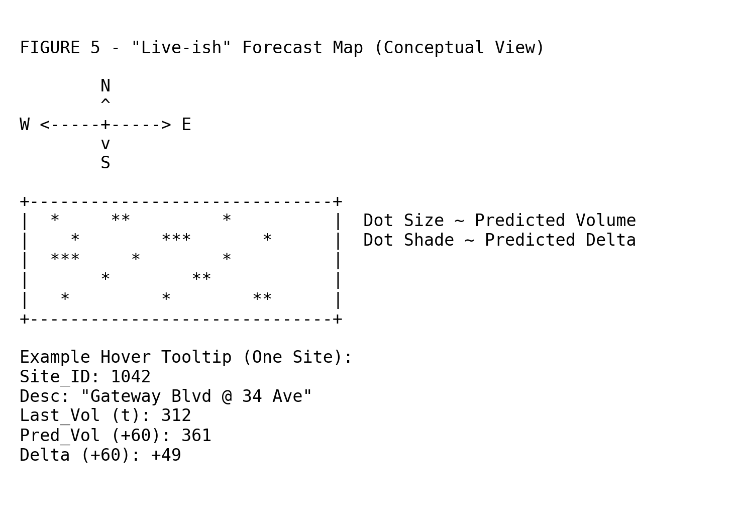
MAP + RANKING
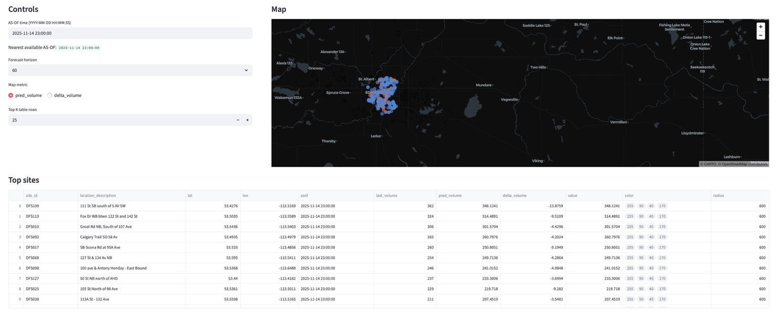
Once the model produced per-site forecasts, I generated outputs for visualization:
- Pick an As-Of time
- Take the last L history steps
- Generate a +60 minute forecast per node
- Write:
- all_site_forecasts.csv
- site_forecasts.geojson
- ranked tables for top predicted volume and top residual delta
The map displays sensor sites as dots, where color/size encode predicted value (or delta). Hover reveals site metadata and forecast values.
This was the only part that felt like an application: not because it was accurate, but because it existed.
LIMITATIONS
- Baseline dominance: short-horizon traffic is largely persistence
- Data window: one month captures periodicity but not rare events
- Graph approximation: geographic kNN is not road topology
- Feature limitation: limited exogenous variables (incidents, weather, events)
- Evaluation scope: MAE over a short window can hide failure modes
CONCLUSION
This project did not produce a useful traffic oracle. It produced a pipeline that runs, forecasts that plot, and a quantitative reminder that many real systems are mostly inertia with brief exceptions.
Two years ago, GNNs were just words. Now they are a word attached to specific bugs, specific baselines, and a specific kind of disappointment.
Traffic is relational. But so is failure: it propagates, it persists, and it looks almost identical to yesterday unless something forces it to change.